From GB to MB - Investigating an Oversized CNN

Inheriting a Black Box

A month into my internship, I was assigned to work on a project involving the identification of Ayurvedic plants from images using a Convolutional Neural Network (CNN).

For readers unfamiliar with the term, a CNN is a type of deep learning model commonly used for image recognition tasks because it learns visual patterns such as edges, textures, and shapes directly from images.

The project was already underway before I joined, so I inherited work that had been developed by previous interns and students. Along with the project, I received a trained CNN model and the dataset it had supposedly been trained on.

At first glance, that sounded sufficient.

It wasn't.

There was no training code. No preprocessing pipeline. No documentation explaining how predictions mapped to plant names. Just a trained model file that was approximately 6.92 GB in size.

To put that into perspective, the model was nearly as large as some local Large Language Models I had downloaded for experimentation.

That immediately raised two questions in my mind:

• What classes was this model actually trained on?
• Why was a CNN this large?

Answering those questions turned into one of the most interesting debugging and optimization journeys I've experienced so far.

Understanding What the Model Was Actually Predicting

Initially, using the model was straightforward.

I could load it, provide an image, and receive a prediction. The problem was that the prediction was simply an integer representing the most likely class.

Prediction: 26

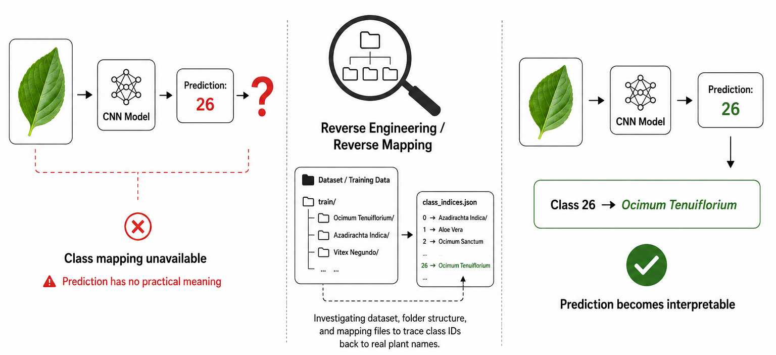
But what exactly was class 26?

Without class mappings, the prediction itself was not particularly useful.

To understand the model better, I performed reverse-mapping on the dataset. By inspecting the dataset structure and examining the ordering of classes, I reconstructed the mapping between class indices and plant names.

For example:

Class 26 → Ocimum Tenuiflorium

As I continued this process, I discovered something unexpected. When I cross-referenced the reverse-mapped labels with our provided physical dataset, the class names simply didn't match. The model had been trained on a completely different set of plant species than the ones we were actually targeting.

The implication was significant: the existing plant data could not be reliably used for the project.

The discovery meant restarting data collection, adding several months to the project timeline. However, identifying the issue early prevented us from training and evaluating future models on incorrect assumptions.

The Bigger Problem: Why Was the Model So Large?

Even after resolving the dataset issue, one question remained.

Why was the model nearly 7 GB?

Most CNN-based image classification models are nowhere near that size. Large models increase storage requirements, deployment costs, and cloud hosting expenses.

A model of this scale would significantly impact infrastructure decisions.

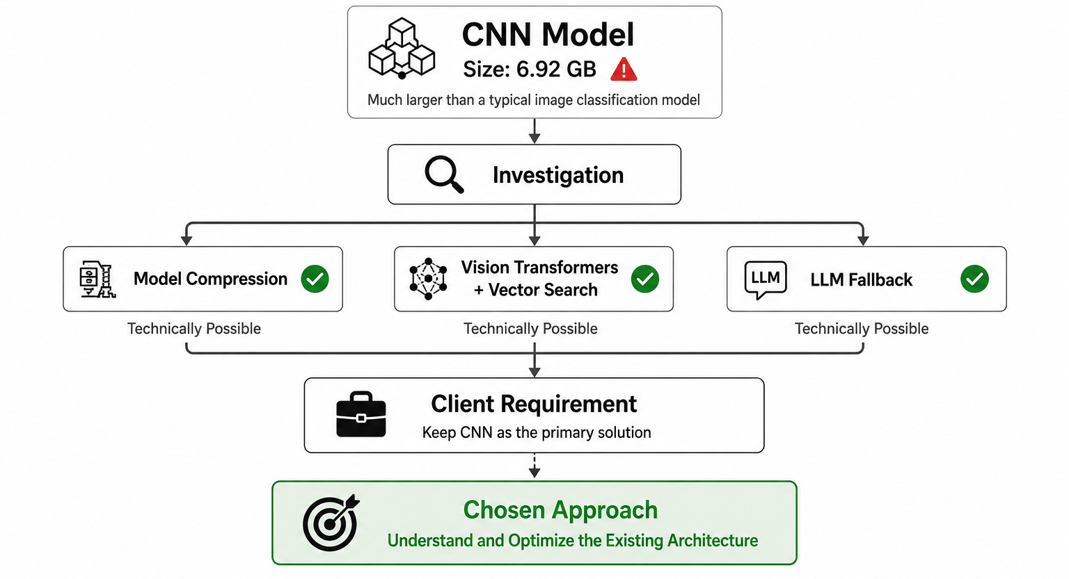
My first assumption was that the issue might be solvable through deployment optimizations rather than architectural changes.

I explored several options:

1. Model compression techniques
2. Alternative classification approaches using Vision Transformers and vector search
3. LLM-assisted fallback mechanisms

Technically, these approaches were interesting.

Practically, they weren't viable.

The client had specifically requested that the CNN model remain the primary solution.

As engineers, we don't always get to choose the ideal technical path. Sometimes the challenge is finding the best solution within the constraints that stakeholders care about.

So instead of replacing the CNN, I decided to understand it.

Going Back to the Source

To investigate further, I requested the original training code and preprocessing pipeline.

Fortunately, the client had maintained good documentation, and the training code was available.

Once I started reviewing the architecture, the source of the problem became apparent.

The issue wasn't the CNN backbone itself.

The issue was a single layer placed immediately after it.

Understanding the Architecture

Before diving into the root cause of the problem, it is worth briefly understanding the architecture being used.

The model was built using Xception (Extreme Inception), a deep convolutional neural network (CNN) architecture developed by Google researchers. It improves upon the standard Inception architecture by replacing traditional convolutions with depthwise separable convolutions, allowing it to achieve high accuracy while remaining computationally efficient.

A CNN learns visual patterns from images, such as edges, textures, shapes, and other distinguishing features. Xception acts as a feature extractor, transforming an input image into a rich set of learned features that can then be used for classification.

Rather than making predictions directly from raw pixel values, the model first uses Xception to identify meaningful visual information from the image. The classification layers that follow then use these extracted features to determine which plant the image most likely belongs to.

In this project, Xception itself was not the source of the problem. The issue originated in the layers that were added after the feature extraction stage.

The Hidden Cost of Flatten()

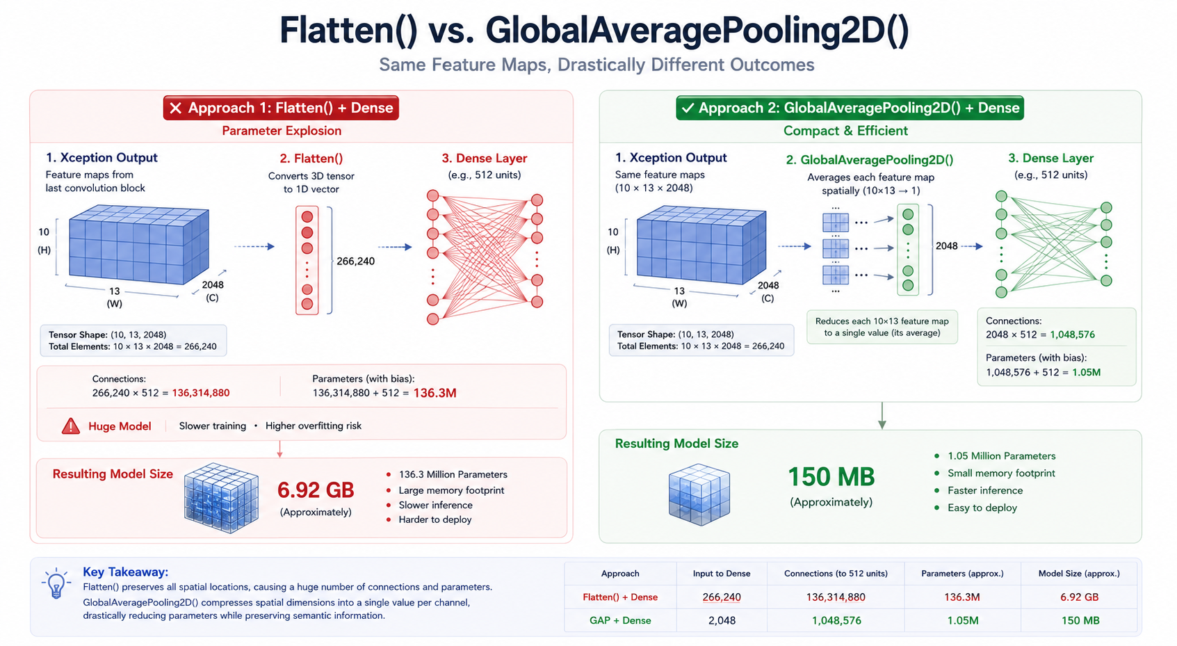
After processing an image, Xception produced an output tensor containing:

• 2048 feature channels
• Each channel sized 10 × 13

That means the output contained:

2048 × 10 × 13
= 266,240 values

At this point, the model applied:

Flatten()

At first glance, Flatten() seems harmless.

All it does is convert multidimensional data into a single long vector.

But that operation can become extremely expensive.

Imagine you have 266,240 values coming out of the CNN.

Flatten() tells the neural network:

Treat every one of these values as an independent input.

Now suppose the next layer is:

Dense(256)

Every one of those 266,240 inputs must connect to each of the 256 neurons.

For simplicity, ignoring bias terms, this creates:

266,240 × 256
= 68,157,440 parameters

This is where the size problem began to reveal itself.

And that's just one dense layer.

Every additional dense layer introduces millions more weights that must be stored in the final model.

The CNN backbone was not the reason the model was huge.

The fully connected layers after Flatten() were.

The architecture was effectively creating a parameter explosion.

A Simpler Alternative: GlobalAveragePooling2D()

While reviewing the architecture, I noticed that the model didn't necessarily need every spatial value coming out of Xception.

What we really cared about was the information captured within each feature channel.

Instead of Flatten(), I replaced it with:

GlobalAveragePooling2D()

The intuition behind GlobalAveragePooling2D() is simple.

Instead of keeping every value from every feature map, it computes a single representative value for each channel.

So instead of:

2048 × 10 × 13
= 266,240 values

we get:

2048 values

One value per channel.

This dramatically reduces the amount of information passed into the dense layers.

Using the same Dense(256) example:

With Flatten():

266,240 × 256
≈ 68 million parameters

With GlobalAveragePooling2D():

2048 × 256
= 524,288 parameters

The difference is enormous.

More importantly, the reduced parameter count often helps models generalize better because there are fewer opportunities to memorize noise in the training data.

Retraining and Measuring the Impact

After making the architectural change, I retrained the model and carefully validated the results.

The outcome was immediately noticeable.

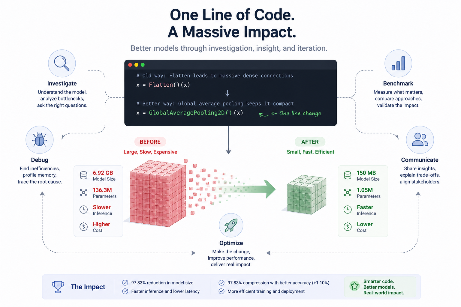
Old Model: ~6.92 GB
New Model: ~150 MB

A reduction of roughly 47×.

But reducing size alone wasn't enough.

A smaller model is only useful if it continues to perform well.

That meant the next step was benchmarking.

Convincing Stakeholders Through Data

One of the most valuable lessons I learned during this project was that technical improvements don't automatically become accepted solutions.

You have to build confidence.

The client was understandably cautious about replacing a model that had already been approved.

Rather than pushing for a completely different approach, I stayed within their comfort zone.

I kept the overall architecture largely familiar and focused on improving the problematic section.

Then I gathered evidence.

Comparing the Models

The original model already had documented evaluation metrics on the test dataset, including:

• Accuracy
• Precision
• Recall
• F1-score
• Macro averages
• Weighted averages
• Per-class performance

I evaluated the new model using the same testing dataset and the same metrics.

Since F1-score is the harmonic mean of precision and recall, I used it as the primary comparison metric while also considering the overall weighted metrics.

The results were:

Metric	Old Model	New Model	Remarks
Model Type	XCEPTION	XCEPTION	Same architecture
Accuracy	98.00%	98.27%	Slight increase
Weighted Precision	98.00%	98.39%	Slight increase
Weighted Recall	97.63%	98.27%	Slight increase
Weighted F1-Score	98.00%	98.24%	Slight increase
Classes with Higher F1	11	11	Equal performance
Classes with Equal F1	18	18	Similar performance
Model Size	6.92 GB	0.15 GB	Significant reduction
Size Reduction	-	97.83%	Major improvement
Compression Ratio	1×	46.13× smaller	Major improvement

The retrained model not only maintained performance but slightly improved it across all major evaluation metrics.

Accuracy increased from 98.00% to 98.27%, while weighted precision, recall, and F1-score also showed modest improvements. This demonstrated that reducing the parameter count through architectural optimization did not negatively impact predictive performance.

Most importantly, these improvements were achieved while reducing the model size from 6.92 GB to approximately 150 MB, resulting in a 97.83% reduction in storage requirements and a compression ratio of over 46×.

From a deployment perspective, the optimized model offered the best of both worlds: comparable or better predictive performance with dramatically lower storage and infrastructure costs.

Lessons Learned

Looking back, this project reinforced several lessons that extend far beyond machine learning.

1. Inherited Systems Deserve Investigation

A working model is not necessarily a well-understood model. Understanding how a system was built can reveal assumptions, risks, and opportunities for improvement.

2. Model Size Is Often an Architectural Problem

Before reaching for compression techniques or infrastructure upgrades, it is worth examining the architecture itself. Sometimes the biggest optimization comes from simplifying the design.

3. Simplicity Can Outperform Complexity

Replacing a single layer had a greater impact than several alternative approaches I explored. The most effective solution was also the simplest.

4. Stakeholder Constraints Matter

Engineering is not only about finding technically elegant solutions. It is about finding solutions that satisfy technical requirements while respecting stakeholder expectations.

5. Benchmarking Builds Trust

Opinions rarely change decisions. Evidence does.

Careful benchmarking and transparent comparisons were ultimately what convinced the client to adopt the new model.

In the end, the most impactful change in this project wasn't a new framework, a new model family, or a complex optimization technique.

It was understanding why a single design decision existed, what impact it had on the architecture, and whether it was still the right choice for the problem being solved.